Recording Excellent Phantom Spectra on the Philips platform

The purpose of this post is to describe our standard process for scanning phantoms, and describe phantom-specific parameters that we use. Acquiring excellent-quality phantom spectra on clinical scanners is a real challenge, which requires a certain amount of witchcraft.

Excellent phantom spectra have narrow lines (~1-2 Hz), so the individual lines of multiplets are resolved, and flat undisturbed baselines to enable accurate phasing and integration.

The first step of acquiring excellent phantom spectra is preparing an excellent phantom (old instructions for a good GABA phantom).

  • Relatively high concentration (~10 mM) is a great start, since phantom experiments often involve parameter series of >10 individual experiments.

  • Sodium azide helps keep the bugs down (and build-up of gunk impacts shimming).

  • Store your phantom in a dark fridge to minimize breakdown, but also know your metabolites (GABA lasts ‘forever’, GSH less well, I think).

  • Use a bottle with friendly geometry that doesn’t result in violent field distortions (we used to use old peanut jars or milk cartons, and they were a lottery on this count). The 1 liter Nalgene bottle style 2125 is fine without being perfect. Spherical containers are better and more contentrated.

  • Avoid air bubbles. It’s better to fill the phantom up (and sacrifice exact concentration) that sacrifice shimmability.

The second step is placement. Try to locate your phantom centrally within the head coil and the main B0 field. A perfect spherical phantom at isocenter in a perfect magnet shouldn’t need shimming, so the closers you can get your ‘cylindrical’ phantom aligned with the central axis of the magnet, the better. If your phantom has an air bubble (most do), it is usually worth tilting the phantom to keep it up one end (ideally in the ‘cap’ region) rather than along the full light of the bottle. Placement judgment and luck in equal measure; sometimes I spend 20 minutes trying to optimize shim and WS on a phantom and just give up. After physically moving it within the bore, I start again.

Even with good shimming, phantoms are less homogeneous than we’d like. Voxel sizes of 2x2x2 cm^3 often yield (noiser) spectra with narrower lines than 3x3x3 cm^3 voxels.

On the Philips system, we use the pb-auto projection-based shimming routine, and it performs well (and quickly) both for phantoms and in vivo. However, you don’t have the option to tweak individual shim currents to optimize the line width manually, so excellent phantom shimming involves an iterative process of slightly moving and/or rotating the voxel, re-running the prep and checking the line width. The reported line width (in the log box) is an imprecise indication, but mostly we rely upon viewing the spectra to check linewidth.

The final piece of the puzzle is water suppression (WS). We tend to use the ‘exc’ option with WS optimization ON for phantom experiments. The automated optimization does a good job of keeping baseline disturbances from residual water signal to a minimum. The quality of WS achievable is dependent on shim quality, and we tend to optimize shim and WS at the same time. Again, sometimes you just can’t get things nice enough, even after moving the voxel around, so you have to reposition the phantom in the scanner. I tend to schedule 30 minutes to get great shim and WS, and then the time to acquire experiments, so 1 hour is never enough to get a full phantom dataset (even when it is technically ‘enough’). Take you time, and get everything just right. This also helps with not mis-entering a parameter series, another common failure mode of phantom experiments!

One final note on chemical shift: your phantom is likely to be at room-temperature and ‘close-to-physiological’ pH. Chemical shifts and coupling constants can depend on temperature (and pH) and for our commonest phantoms the water line tends to come at ~4.8 ppm. For frequency-selective experiments like edited MRS, you need to account for this in setting editing pulse frequencies. This is handled in our patch via the BASING parameter ‘water freq’. The scanner tends to assume the water line comes at 4.68 ppm, so we can infer the correct water shift from a processed spectrum by checking how far off-resonance the metabolite signals appear in teh SpectroView window.
Optimizing Voxel geometry on the Philips platform

One common artifact that we see in MR spectra are unwanted water echoes. The spectrum below shows this behavior around 4 ppm. It manifests as a region of the spectrum with ‘locally increased noise’, which is more accurately considered as a broad signal with a large first-order phase error.

Screen Shot 2021-03-29 at 11.24.24 AM.png

This happens when the sequence accidentally refocuses water signals from outside of voxel OOV (or merely fails to fully suppress them with the gradient pulses), and can seriously interfere with quantification. For a given brain location and acquisition protocol, these artifacts are relatively consistent and so can be ‘optimized away ‘. This process is something we advise collaborators to do every time they set up a protocol for a new brain region.

The key parameters are the voxel orientation (transverse/coronal/sagittal) which changes the ordering of the slice-selective pulses within the PRESS sequence (or rotates the experiment 90 degrees about a cube-face) and the water-fat shifts (L/R etc) which flip the slice-selective gradients one-by-one (reflecting the experiment spatially a plane parallel to a cube-face).

Before you work on a challenging brain region, make sure your sequence works in PCC or some other ‘easy’ region with which you have experience. When you are sure the sequence is set up correctly, then you can move onto this geometric optimization.

Step 1: Run an in vivo scan in a new brain region. Use 320 averages and ~25ml volume so you know what to expect in terms of SNR. If the spectrum looks ‘clean’ with respect to these OOV echoes, then I would not continue with this process. Run a new subject and hopefully that’ll look fine too.

Step 2: If you see OOV echoes, run scans with all three options of the orientation parameter, and select the one that gives the smallest OOV echoes.

Step 3: With that orientation, start working on the water-fate shifts. One quick option is to flip all three and see if it solves your problem. Hopefully you can see the OOV echoes in the Spectroscopy tool on the scanner. For each water-fat axis, select the option that gives the smallest OOV echoes.

This process is not 100% reproducible across subjects, but it is enough to be useful.

Screen Shot 2021-03-29 at 11.23.44 AM.png

One final note: The data above were acquired from this midline ACC voxel. The orange box corresponds to the 3 ppm signal and the white to the chemical-shift-displaced water signal. When setting up a new voxel location, I tend to recommend setting the water-fat shifts to put the white box ‘inside‘ the orange box. By ‘inside’, I mean away from scalp and other challenging areas.. towards the middle of the brain….

Processing phantom data through Gannet

Some Gannet users have asked us whether Gannet can process phantom data. The answer is yes! Gannet can load and fit phantom data for GABA, GSH, Glx, Lac, and EtOH edited data acquired either by MEGA-PRESS or HERMES.

Note that to quantify your measurements you will need to also have an unsuppressed water signal acquisition to use as a concentration reference.

For example, the following steps would allow you to process and quantify example Lac-edited phantom data acquired on a Siemens scanner:

  1. Download the latest version of Gannet.

  2. Open GannetPreInitialise.m and make sure the settings match the screenshot in Figure 1 below, making sure MRS_struct.p.phantom is set to 1.

  3. Save your changes and enter the directory containing your phantom data.

  4. Run GannetLoad using the following command (see the output in Figure 2):

    GannetLoad({'meas_MID00380_FID11555_UNIV_Lac_TE140_22ms_1024_1khz.dat'},{'meas_MID00382_FID11557_UNIV_Lac_TE140_H20.dat'});
  5. Then run GannetFitPhantom to fit and quantify the edited Lac signal (see the output in Figure 3):

    MRS = GannetFitPhantom(MRS);

Figure 1

Figure 2

Figure 2

Figure 3

Figure 3

Hackathon Live Update Stream

Non-Live webcam feed!

Non-Live webcam feed!

455PM: A quick summary: We haven't come up with a method that makes things better. BUT, we have learned several important things:

1. NAA-based correction can do a lot to clean up the GSH-diff spectrum. 

2. Metrics matter.  By taken a mean 'quality score', we shot ourselves in the foot. We will reassess all data based on median, and maybe normalized by the group average SD subtraction artifacts, not within-subject... 

255PM: Bumped out of the large conference room.

1239PM: In terms of actual progress. We have tested 6 methods. None of them do very well. Onwards and upwards!

1200PM: Pizza arrives as ably planned by Mark (picking up from the organizational travesty that was Nick's lunch arrangement).  

933AM: Donutgate: the number of declared donuts doesn't match the number of eats donuts.

930AM: Donut scores: Georg 2 Nick 2 Richard 2 Ashley 1 Muhammad 0 Tao 1 Kim 1 Mark 1

922AM: Nick just left the room. Minus 70 Edden points.

920: Pretend to set up a live webcam feed.

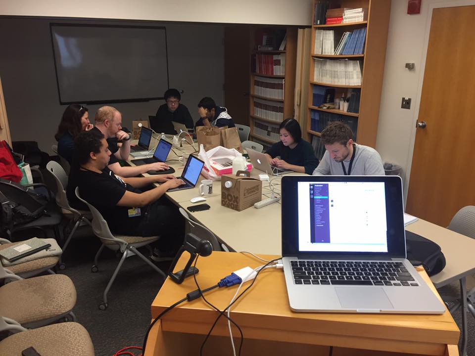
905AM: Preliminary chat over.  Repositories forked and coding has begun. 

840AM: Skype to Jamie Near in Canada.

755AM: Room setup. Do we have enough extension leads? 

730AM: Dunkin' Donuts stop for fuel.

559AM: I remembered to grab my charged-overnight laptop on the way out of the house. A good start.

Frequency Correction Hackathon February 23 2015

The alignment of editing-ON and editing-OFF scans is an issue for all J-difference-edited MRS, but especially for HERMES editing, where at least four sub-experiments (with different signal characteristics) must be aligned.  

We are going to be taking a shotgun approach to improving frequency-and-phase correction for HERMES.  Tomorrow, we will focus on HERMES of GABA and GSH, trialling a (hopefully large) number of methods on 4x10 subjects in vivo data (collected at three sites) and simulated data.  We will implement the best method(s) in Gannet and hope to publish the results soon after.